5. Transport module: RMC|Transport

RMC|Transport is a module within the RMC model family focused on the transportation sector, designed to analyze supply-demand dynamics, technology and energy mix, carbon emissions, and other impacts (such as critical metal demand) during the low-carbon transition of China’s transportation sector. Different from the main RMC model, the transportation module employs a stock-flow system dynamics approach. Its geographical coverage includes 31 provincial-level administrative units in mainland China. It incorporates, in a bottom-up manner, major key technological information, energy consumption and GHG emissions relevant to the transportation sector, and has been calibrated based on historical data for vehicle stocks, activity levels, and technology costs.

5.1. Model structure

As shown in Fig. 5-1, RMC|Transport primarily covers the road transport sector (with future extensions planned for shipping, rail, and other transport sectors). This includes private vehicles, commercial vehicles, public service vehicles, and other road transport. The energy types considered in the model include gasoline, diesel, electricity, hydrogen, natural gas, and other alternative fuels.

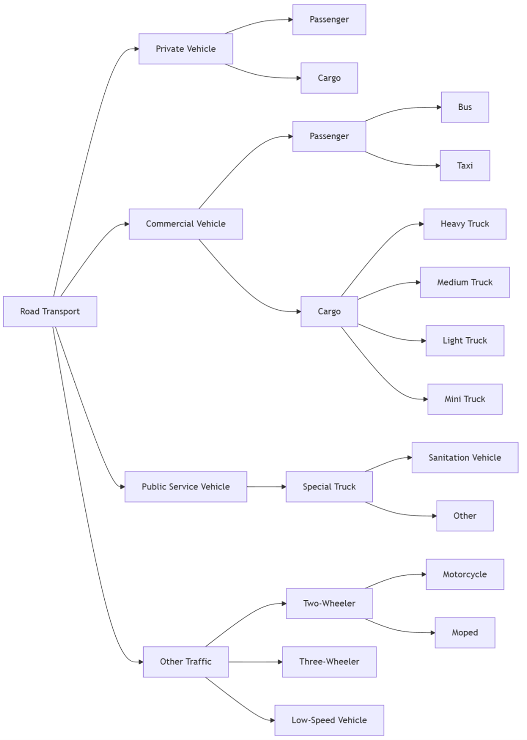
Fig. 5-1: Modeled road transport sector.

5.2. Modelling vehicle stocks and flows

The model utilizes a system dynamics approach to analyze the stock-flow relationships of private passenger cars. Let \(V_{f,c,a}(t)\) denote the stock of private passenger cars in year \(t\), with fuel type \(f\), vehicle type \(c\), and vehicle age \(a\). Aggregating over age groups gives \(V_{f,c}(t)=\sum_{a=0}^A V_{f,c,a}(t)\). The total stock \(N(t)\) is defined as the sum of stocks across all fuel-body type combinations, i.e., \(N(t)=\sum_{f,c}V_{f,c}(t)\).

Denoting the new registrations of private passenger cars in year t as \(n_{f,c}(t)\), and the number of vehicles retired due to reaching end-of-life as \(r_{f,c,a} (t)\), the stock-flow relationship is expressed as:

\[ \Delta V_{f,c}(t)=n_{f,c} (t)-\sum_{a=0}^A r_{f,c,a} (t) \tag{5-1} \]

where the retirements satisfy:

\[ r_{f,c,a}(t)=\alpha_{f,c,a} (t)\cdot V_{f,c,a} (t)\tag{5-2} \]

Here, \(\alpha_{f,c,a}(t)\in[0,1)\) is the retirement risk coefficient for the specific vehicle type.

The national per capita private passenger car stock \(\bar{N}(t)\) follows a GDP-enhanced Gompertz curve:

\[ \bar{N}(t)=\gamma_{max}\cdot \text{exp}(-K\cdot \text{exp}(-B\cdot G(t)))+\theta\cdot \bar{N}(t-1)\tag{5-3} \]

where \(\gamma_{max}\) is the saturation level, \(G(t)\) is the per capita GDP, positive constants \(K\) and \(B\) are the shape and location parameters of the curve, respectively, and the coefficient \(\theta\in [0,1]\) adjusts for the inertia effect of the per capita stock and the income effect. Based on this, the absolute stock level \(N(t)\) is obtained using the population \(POP_t\):

\[ N(t)=\bar{N}(t)\cdot POP_t\tag{5-4} \]

To ensure consistency between macro and micro levels, the annual net change in the private passenger car stock \(\Delta N_t=N(t+1)-N(t)\), the total new registrations \(n_t=\sum_{f,c}n_{f,c}(t)\), and the total retirements \(R_t=\sum_{f,c,a}r_{f,c,a}(t)\) must satisfy:

\[ \Delta N_t=n_t-R_t\tag{5-5} \]

At the fleet level, the recursive relationship with a one-year time step is as follows:

\[ V_{f,c,a+1}(t+1)=(1-\alpha_{f,c,a}(t))\cdot V_{f,c,a}(t), \forall a≥0\tag{5-6} \]

\[ V_{f,c,0}(t+1)=n_{f,c}(t)\tag{5-7} \]

Vehicle lifetime is assumed to follow a Weibull distribution to reflect the empirical pattern that older vehicles are retired more frequently. The retirement risk coefficient can then be calculated from the Weibull distribution parameters:

\[ \alpha_{f,c,a}=1-\frac{S(a+1)}{S(a)} =1-exp\left(-\left[\left(\frac{a+1}{h_{f,c}}\right)^{s_{f,c}}-\left(\frac{a}{h_{f,c}}\right)^{s_{f,c}}\right]\right)\tag{5-8} \]

Alternatively, log-normal or Gamma distributions can be used for simplification.

The projection results for the ownership of private passenger cars are shown in Fig. 5-2. Currently, the number of private passenger cars per 100 people shows a significant positive correlation with economic development levels. Economically developed regions like Zhejiang, Jiangsu, and Beijing all exceed 24 vehicles per 100 people, while provinces such as Jiangxi, Hunan, and Gansu have approximately 15 vehicles per 100 people. In the future, the growth of the car stock in first-tier cities is projected to be slower, approaching or reaching saturation levels after 2050, while other regions will maintain relatively faster growth rates.

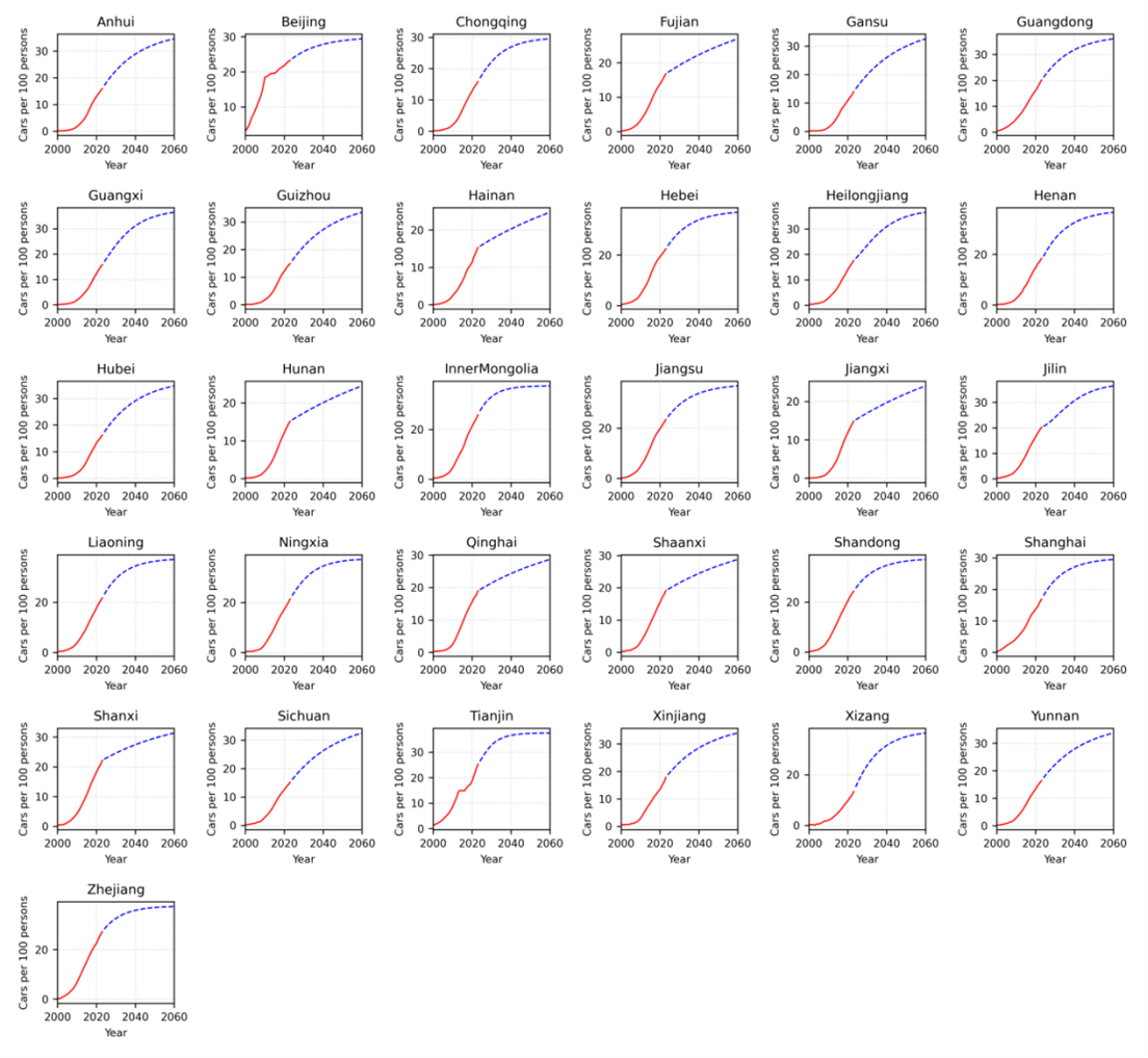
Fig. 5-2: Ownership of private passenger cars per 100 inhabitants by province (2000-2060).

5.3. Consumer choice for private passenger vehicles

The selection of private passenger cars is driven by multiple factors, primarily including the vehicle purchase price, per-100-kilometer energy cost, driving range, and refueling/recharging convenience. These factors collectively shape consumer decision-making behavior, and their interrelationships are illustrated in Fig. 5-3.

Fig. 5-3: Main factors influencing the choice of private passenger vehicles.

5.3.1. Vehicle purchase price

The vehicle purchase price refers to the total cost actually paid by the consumer, encompassing the Manufacturer’s Suggested Retail Price (MSRP), the influence of policy incentives, and market conditions. The final price paid by the consumer equals the sum of the MSRP, insurance, and license plate costs, minus dealer discounts, local subsidies, and consumption vouchers.

The evolution of this parameter is primarily driven by local government subsidy policies (e.g., national and local subsidies) and license plate costs in cities with purchase restrictions. Provincial-level discount coefficients for BEVs and PHEVs are set based on historical data (implementation of subsidy policies from 2017 to 2021). For instance, the local subsidy was approximately one thirds the national subsidy in 2019 and 10% in 2020, respectively, and phased out to zero in 2021. Future price pathways are described using the price change rate parameter \(\delta_{i,f}\):

\[ P_f(t)=P_f(t_0)\cdot\Pi_{i=t_0}^t (1+\delta_{i,f})\tag{5-9} \]

where \(P_f (t)\) is the purchase price of a vehicle of fuel type \(f\) in period \(t\), and \(P_f (t_0)\) is the purchase price of that vehicle type in the base year.

Table 5-1: Phased change trend of purchase price.

Fuel Type	2025–2030	2030–2045	2045–2060
BEV	Rapid decline (battery cost-driven)	Stabilization or slow decline (marginal improvements)	Most affordable
PHEV	Slight decline (dependent on dual systems)	Remains basically stable	Demand decreases → Price rebounds or product exits market
GASL	Remains stable or increases slightly	Accelerated increase (rising environmental costs)	Sharp decrease → Price structure becomes
DIESEL	Slight increase (due to restrictions)	Significant increase (ban on sales/use)	Basically exits the market

Table 5-2: Price change rate of different fuel types.

Fuel Type	2025–2030	2030–2045	2045–2060
BEV	–5%/yr	–1.5%/yr	–0.5~0%/yr
PHEV	–2%/yr	0%/yr	1%/yr
GASL	0~1%/yr	2%/yr	3~4%/yr
DIESEL	1%/yr	4%/yr	5%/yr

5.3.2. Fuel efficiency

Vehicle fuel efficiency is measured by the monetary value of energy consumed per 100 km driven. For BEVs, it is the product of electricity consumption per 100 km and the electricity price; for gasoline/diesel vehicles (GASL/DIESEL), it is the product of fuel consumption per 100 km and the fuel price; for PHEVs, a comprehensive calculation is required. The formula is as follows:

\[ C_{p,k} (t)=EC_{p,k} (t)\cdot\alpha_{p,k}\cdot P_{p,k}^{\text{fuel}}(t)\tag{5-10} \]

Here, \(C_{p,k} (t)\) is the cost for province \(p\) and vehicle type \(k\) in period \(t\), \(EC_{p,k} (t)\) is the NEDC standard energy consumption, \(\alpha_{p,k}\) is a province-specific adjustment coefficient, and \(P_{p,k}^{\text{fuel}} (t)\) is the fuel price per unit. BEV energy efficiency is modeled based on an S-curve technological diffusion path derived from IEA physical limits. Fuel consumption for internal combustion engine vehicles remains stable. PHEV fuel consumption is constant, with efficiency improvements relying on increased electric range. Fuel price evolution is based on a green transition scenario: electricity prices first rise, then fall due to renewables, while oil prices experience a long-term moderate increase due to carbon taxes.

5.5.5. Driving range

Driving range refers to the maximum distance a vehicle can travel on a full energy supply and is a key consideration for NEV users. The range for conventional vehicles is assumed constant. The range for NEVs is determined by cell energy density \(ED_{f=\text{NEV}} (t)\), battery pack mass \(M_{\text{pack}}\), battery pack integration efficiency \(\eta_{\text{pack}} (t)\), and energy consumption \(EC_{p,f=\text{NEV}}(t)\cdot \alpha_{p,f=\text{NEV}}\):

\[ Range_{p,f=\text{NEV}} (t)=\frac{ED_{p,f=\text{NEV}} (t)\cdot M_{\text{pack}}\cdot \eta_{\text{pack}} (t)}{EC_{p,f=\text{NEV}} (t)\cdot\alpha_{p,f=\text{NEV}}}\times 100\%\tag{5-11} \]

The industry average cell energy density \(ED_{\text{avg}}(t)\) is the market-share-weighted average of different technology pathways:

\[ ED_{\text{avg}}(t)=\sum_{\varphi}s_{\varphi}(t)\cdot ED_{\varphi}(t)\tag{5-12} \]

Here, \(s_{\varphi}(t)\) is the market share of technology \(\varphi\) (e.g., NMC, LFP, Li-S/Li-Air), and the specific energy density \(ED_{\varphi}(t)\) follows an S-curve of technological progress.

5.3.4. Refueling/Recharging convenience

Refueling/recharging convenience quantifies infrastructure accessibility and is crucial for NEV adoption. The convenience index for each province is defined by the ratio of infrastructure density to vehicle stock:

\[ ERAI_{p,f}(t)=\frac{RI_{p,f}(t)/Area_p}{V_{p,f}(t)}\tag{5-13} \]

Where \(RI_{p,f}(t)\) is the number of refueling/recharging facilities (e.g., charging points, gas stations), \(Area_p\) the provincial area, and \(V_{p,f}(t)\) is the vehicle ownership. Convenience for BEV is measured by the ratio of public charging point density to BEV stock; convenience for ICEV is measured by the ratio of gas station density to total ICEV ownership; convenience for PHEV considers the ratio combining private charging point density (relative to PHEV stock) and gas station density. The evolution of the vehicle-to-infrastructure ratio follows national planning targets. The ratio between public and private charging points, \(\Psi_p (t)\), is defined by system consistency constraints:

\[ \frac{1}{R_{\text{public}}} = \frac{V_{p,f=\text{BEV}}(t) + V_{p,f=\text{PHEV}}(t)}{Charge_{\text{public}_p}(t)} \tag{5-14} \]

\[ \frac{1}{R_{\text{private}}} = \frac{V_{p,f=\text{BEV}}(t) + V_{p,f=\text{PHEV}}(t)}{Charge_{\text{private}_p}(t)} \tag{5-15} \]

\[ \frac{1}{R_{\text{total}}} = \frac{V_{p,f=\text{BEV}}(t) + V_{p,f=\text{PHEV}}(t)}{Charge_{\text{public}_p}(t) + Charge_{\text{private}_p}(t)} \tag{5-16} \]

\[ \frac{1}{R_{\text{total}}} = \frac{1}{R_{\text{public}}} + \frac{1}{R_{\text{private}}} \tag{5-17} \]

\[ \Psi_p(t) = \frac{R_{\text{public}_p}(t)}{R_{\text{private}_p}(t)} \tag{5-18} \]

5.4. Projection for buses and taxis

The projection for the public bus and taxi stock uses a demand-driven capacity planning model, implemented in three steps.

Predicting Public Transport Passenger Volume: Provincial public transport passenger volume is projected using multiple linear regression based on population, GDP per capita, and private car ownership. Regarding historical data, statistics before 2017 included buses/taxis and rail transit; post-2018 data are reported separately; from 2020, taxi and ferry passenger volumes are included. These changes are considered in our estimation.

Estimating Bus/Taxi Share: The variable ‘share of bus/taxi passenger volume’ is constructed. Its future trend is estimated using machine learning methods based on its historical nonlinear relationship with urbanization rates. This share is assumed to change dynamically with urbanization, considering factors like new subway line openings (e.g., assumed for Qinghai, Tibet around 2030).

Deriving Vehicle Stock from Service Intensity: The vehicle stock is derived using provincial ‘service intensity’ (passengers carried per vehicle per year). Service intensity is obtained by fitting the relationship between annual passenger volume and the number of operational vehicles over the past five years, using a weighted average method. The future vehicle stock is then calculated based on the projected passenger volume and this service intensity.

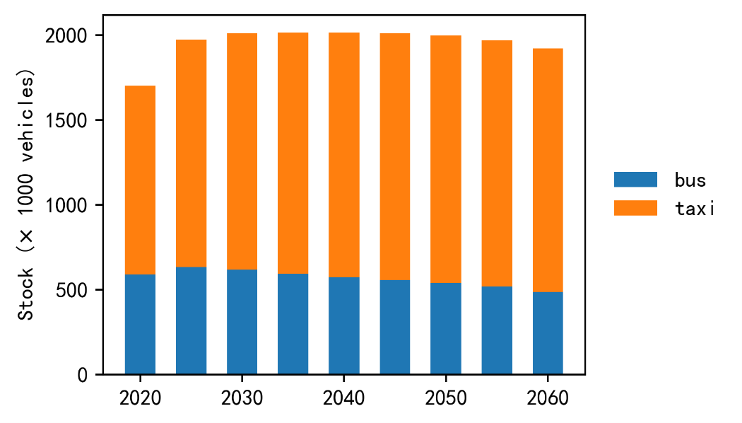
Fig. 5-4: National bus and taxi stock forecast (2020-2060).

Table 5-3: Regional grouping based on subway availability.

Group	Description	Region
G1	Subway opened early (<1997)	Beijing, Shanghai
G2	Subway not yet opened (as of 2023)	Hainan, Qinghai, Tibet, Ningxia
G3	Subway opened between 1997-2005	Guangdong, Tianjin, Hubei, Jilin, Liaoning, Jiangsu, Chongqing
G4	Subway opened between 2009-2014	Sichuan, Henan, Heilongjiang, Zhejiang, Hunan, Shaanxi, Yunnan
G5	Subway opened in 2015	Fujian, Jiangxi, Shandong
G6	Subway opened between 2016-2021	Inner Mongolia, Anhui, Hebei, Guangxi, Gansu, Guizhou, Xinjiang, Shanxi